# make repeatable
set.seed(42)
# get 100 values from normal
x <- rnorm(100)1 Installing R
In this class, we will be using R to perform statistical analyses. R is a free software program designed for use in a myriad of statistical and computational scenarios. It can handle extremely large datasets, can handle spatial data, and has wrappers for compatibility with Python, Bash, and other programs (even Java!).
1.1 Setup
First, we need to download R onto your machine. We are also going to download RStudio to assist with creating R scripts and documents.
1.1.1 Installing R
First, navigate to the R download and install page. Download the appropriate version for your operating system (Windows, Mac, or Linux). Note that coding will be formatted slightly different for Windows than for other operating systems. If you have a Chromebook, you will have to follow the online instructions for installing both programs on Chrome.
Follow the installation steps for R, and verify that the installation was successful by searching for R on your machine. You should be presented with a coding window that looks like the following, but may not be an exact match:
R version 4.4.1 (2024-06-14) -- "Race for Your Life"
Copyright (C) 2024 The R Foundation for Statistical Computing
Platform: aarch64-apple-darwin20

R is free software and comes with ABSOLUTELY NO WARRANTY.
You are welcome to redistribute it under certain conditions.
Type 'license()' or 'licence()' for distribution details.

  Natural language support but running in an English locale

R is a collaborative project with many contributors.
Type 'contributors()' for more information and
'citation()' on how to cite R or R packages in publications.

Type 'demo()' for some demos, 'help()' for on-line help, or
'help.start()' for an HTML browser interface to help.
Type 'q()' to quit R.

>
If that screen appears, congratulations! R is properly installed. If the install was not successful, please talk to your instructor and teaching assistant(s) for help with installation.
1.1.2 Installing RStudio
RStudio is a GUI (graphics user interface) that helps make R easier to use. Furthermore, it allows you to create documents in R, including websites (such as this one), PDFs, and even presentations. This can greatly streamline the research pipeline and help you publish your results and associated code in a quick and efficient fashion.
Head over the the RStudio download website and download “RStudio Desktop”, which is free. Be sure to pick the correct version for your machine.
Open RStudio on your machine. You should be presented with something like the following:
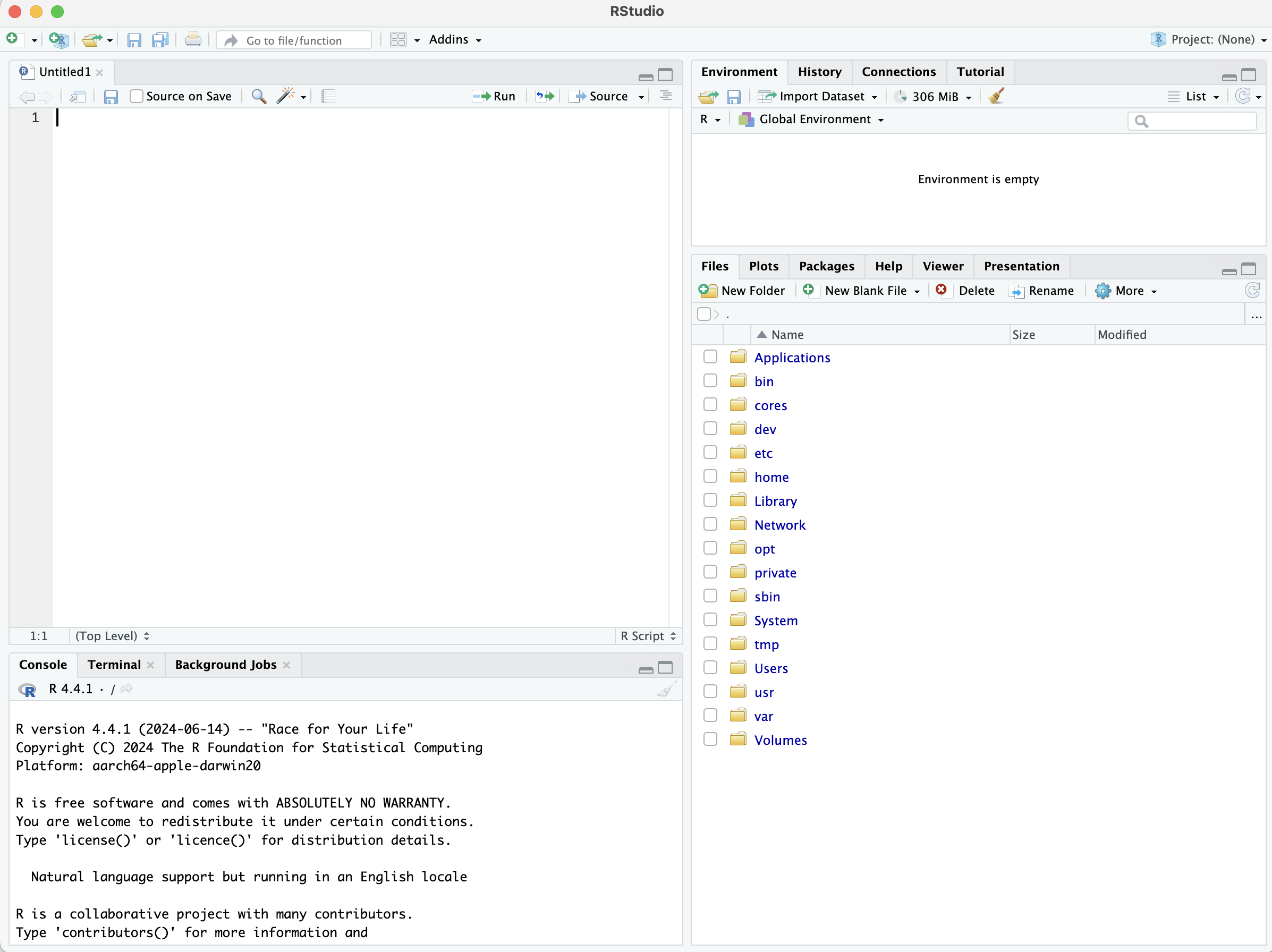
In RStudio, the top left window is always going to be our coding window. This is where we will type all of our code and create our documents. In the bottom left we will see R executing the code. This will show what the computer is “thinking” and will help us spot any potential issues. The top right window is the “environment”, which shows what variables and datasets are stored within the computers’ memory. (It can also show some other things, but we aren’t concerned with that at this point). The bottom right window is the “display” window. This is where plots and help windows will appear if they don’t appear in the document (top left) window itself.
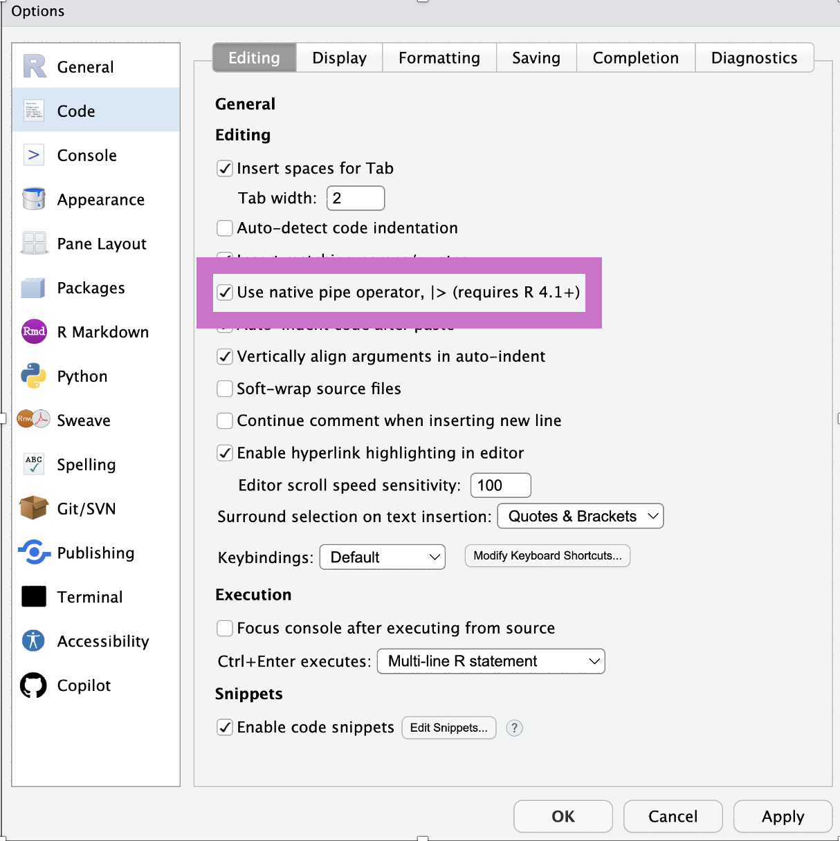
1.1.3 Setting up the “native pipe” operator
There are two ways to type commands in R: in a “nested” fashion and in a “piped” fashion. We will be using the “piped” fashion for ease of use.
In RStudio, click on the tabs at the top of the screen to go to Tools > Global Options, and in the pop up screen select Code. On this screen, you should see a tick box for “Use native pipe operator”. Make sure this box is checked. Now, we can use CTRL + SHIFT + M (a.k.a., ^ + SHIFT + M on Mac) to insert the “pipe” operator |>.
1.1.3.1 Using |> pipes
Let’s say that we have a random series of 100 numbers from a random normal distribution, which we can get by copying and running the following in the lower left coding window:
We want to get the mean of these values and round these values to two decimal places for our final answer. To do this in a nested fashion, we would do the following:
# round mean of x
round(mean(x), 2)
[1] 0.03Note that we call this the “nested” method because one command (mean) is located inside another command (round). This is fine for short series of commands, but can get confusing when too many commands are combined. Thus, we can use the |> pipe method instead.
The pipe operator takes whatever came previously and puts it through the next command. For example, mean(x) could also be written as x |> mean(), where x would be placed inside of mean().
# take x
x |>
  # get mean
  mean() |>
  # round answer
  round(2)
[1] 0.03As you can see, the above breaks things down into a more step-by-step fashion, and makes code easier to follow. We will be using this extensively in this course.
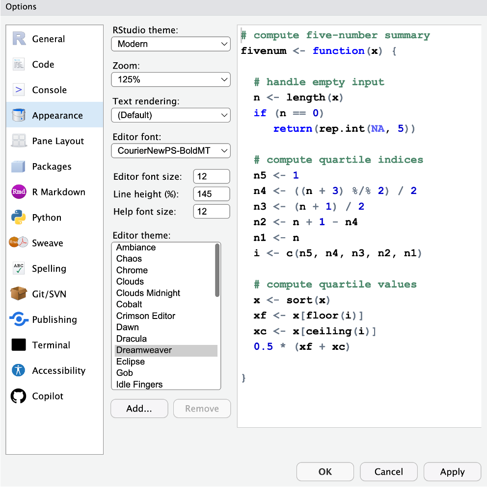
1.1.4 Customizing R
RStudio’s interfacecan be customized within the global options under “appearance”. You can explore different fonts, different font sizes, and different color schemes. Please choose one that makes it easy for you to:
- Has a color scheme that makes the difference between different commands, numbers, and objects easy to see and is easily readable for you.
- Has a font that is a type and size that is easily readable for you.
1.2 PDF Compatability
In order to make pdf documents, you will need to have a tinytex distribution installed. You can do this with the following commands in the console (bottom left) window.
install.packages('tinytex')
tinytex::install_tinytex()