10  χ2 (Chi-squared) tests

10.1 \(\chi^2\)-squared distribution

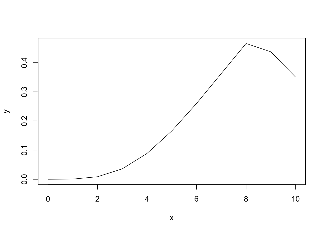
\(\chi^2\)-squared (pronounced “kai”, and spelled “chi”) is a distribution used to understand if count data between different categories matches our expectation. For example, if we are looking at students in the class and comparing major vs. number of books read, we would expect no association, however we may find an association for a major such as English which required reading more literature. The \(\chi^2\) introduces a new term degrees of freedom (\(df\)) which reflects the number of individuals in the study. For many tests, \(df\) are needed to reflect how a distribution changes with respect the number of individuals (and amount of variation possible) within a dataset. The equation for the \(\chi^2\) is as follows, with the \(\chi^2\) being a special case of the gamma (\(\gamma\) or \(\Gamma\)) distribution that is affected by the \(df\), which is defined as the number of rows minus one multiplied by the number of columns minus one \(df = (rows-1)(cols-1)\):

\[ f_n(x)=\frac{1}{2^{\frac{n}{2}}\Gamma(\frac{n}{2})}x^\frac{n}{2-1}e^\frac{-x}{2} \]

The \(\chi^2\)-squared distribution is also represented by the following functions, which perform the same things as the previous outlined equivalents for Poisson and binomial:

• dchisq

• pchisq

• qchisq

• rchisq

We can view these probabilities as well:

x <- 0:10

y <- pchisq(x, df = 9)

# any value greater than 0.5 is subtracted from 1
y[y > 0.5] <- 1 - y[y > 0.5]

plot(x,y,type="l")

10.1.1 Calculating the test statistic

We evaluate \(\chi^2\) tests by calculating a \(\chi^2\) value based on our data and comparing it to an expected \(\chi^2\) distribution. This test statistic can be evaluated by looking at a \(\chi^2\) table or by using R. Note that you need to know the degrees of freedom in order to properly evaluate a \(\chi^2\) test. We calculate our test statistic as follows:

\[ \chi^2=\Sigma\frac{(o-e)^2}{e} \]

where \(e =\) the number of expected individuals and \(o =\) the number of observed individuals in each category. Since we are squaring these values, we will only have positive values, and thus this will always be a one-tailed test.

There are multiple types of \(\chi^2\) test, including the following we will cover here:

• \(\chi^2\) Goodness-of-fit test

• \(\chi^2\) test of independence

10.1.2 \(\chi^2\) goodness-of-fit test

A \(\chi^2\) goodness-of-fit test looks at a vector of data, or counts in different categories, and asks if the observed frequencies vary from the expected frequencies.

10.1.2.1 \(\chi^2\) estimate by hand

Let’s say, for example, we have the following dataset:

Hour	No. Drinks Sold
6-7	3
7-8	8
8-9	15
9-10	7
10-12	5
12-13	20
13-14	18
14-15	8
15-16	10
16-17	12

Now, we can ask if the probability of selling drinks is the same across all time periods.

drinks <- c(3, 8, 15, 7, 5, 20, 18, 8, 10, 12)

We can get the expected counts by assuming an equal probability for each time period; thus, \(Exp(x)=\frac{N}{categories}\).

# sum all values for total number
N <- sum(drinks)

# get length of vector for categories
cats <- length(drinks)

# repeat calculation same number of times as length
exp_drinks <- rep(N/cats, cats)

exp_drinks

 [1] 10.6 10.6 10.6 10.6 10.6 10.6 10.6 10.6 10.6 10.6

Now, we can do out \(\chi^2\) calculation.

chi_vals <- ((drinks - exp_drinks)^2)/exp_drinks

chi_vals

 [1] 5.44905660 0.63773585 1.82641509 1.22264151 2.95849057 8.33584906
 [7] 5.16603774 0.63773585 0.03396226 0.18490566

sum(chi_vals)

[1] 26.45283

And now, to get the probability.

chi_vals |> 
  # get chi statistic
  sum() |> 
  # get p value
  pchisq(df = length(chi_vals) - 1,
         # looking RIGHT
         lower.tail = F)

[1] 0.001721825

Here, we get \(p = 0.002\), indicating that there is not an equal probability for selling drinks at different times of day.

10.1.2.2 \(\chi^2\) estimation by code

We can use the test chisq.test to perform this analysis as well.

chisq.test(drinks)

    Chi-squared test for given probabilities

data:  drinks
X-squared = 26.453, df = 9, p-value = 0.001722

As we can see, these values are exactly the same as we just calculated by hand! Note that we can define the probability p if we want, otherwise it defaults to p = rep(1/length(x), length(x)).

10.1.3 \(\chi^2\) test of independence

Usually when we use a \(\chi^2\), we are looking at count data. Let’s consider the following hypothetical scenario, comparing experience with R between non-biology majors (who, in this theoretical scenario, do not regularly use R) and Biology majors who are required to take R for this class:

The above table of counts is also known as a contingency table. Intuitively, we can see a difference, but we want to perform a statistical test to see just how likely these counts would be if both groups were equally likely. We can calculate this both “by hand” and using built in R functions.

Major	R experience	No R experience
Non-biology	3	10
Biology	9	2

10.1.3.1 \(\chi^2\) estimations by hand

First, we can enter the data into R.

data <- matrix(data = c(3,10,9,2), nrow = 2, ncol = 2, byrow = T)

colnames(data) <- c("R", "No R")
rownames(data) <- c("Non-biology", "Biology")

data

            R No R
Non-biology 3   10
Biology     9    2

Next, we need the observed - expected values. We determine expected values either through probability (\(0.5 \cdot n\) for equal probability for two categories) or via calculating the the expected values (see later section on expected counts). In this case, since we are looking at equally likely in each cell, we have an expected matrix as follows:

# total datapoints
N <- sum(data)

expected <- matrix(data = c(0.25*N,0.25*N,0.25*N,0.25*N), nrow = 2, ncol = 2, byrow = T)

colnames(expected) <- c("R", "No R")
rownames(expected) <- c("Non-biology", "Biology")

expected

            R No R
Non-biology 6    6
Biology     6    6

Now we need to find our observed - expected.

o_e <- data - expected

o_e

             R No R
Non-biology -3    4
Biology      3   -4

Note that in R we can add and subtract matrices, so there’s no reason to reformat these data!

Now, we can square these data.

o_e2 <- o_e^2

o_e2

            R No R
Non-biology 9   16
Biology     9   16

Next, we take these and divide them by the expected values and then sum those values.

chi_matrix <- o_e2/expected

chi_matrix

              R     No R
Non-biology 1.5 2.666667
Biology     1.5 2.666667

sum(chi_matrix)

[1] 8.333333

Here, we get a \(\chi^2\) value of 8.3333333. We can use our handy family functions to determine the probability of this event:

chi_matrix |> 
  # get chi statistic
  sum() |> 
  pchisq(df = 1,
         # looking RIGHT
         lower.tail = F)

[1] 0.003892417

Here, we get a \(p\) value of:

chi_matrix |> 
  sum() |> 
  pchisq(df = 1, lower.tail = F) |> 
  round(3)

[1] 0.004

Alternatively, we can calculate this using expected counts. For many situations, we don’t know what the baseline probability should be, so we calculate the expected counts based on what we do know. Expected counts are calculated as follows:

\[ Exp(x)=\frac{\Sigma(row_x)\cdot\Sigma(col_x)}{N} \]

where \(N\) is the sum of all individuals in the table. For the above example, this would look like this:

data_colsums <- colSums(data)
data_rowsums <- rowSums(data)
N <- sum(data)

expected <- matrix(data = c(data_colsums[1]*data_rowsums[1],
                            data_colsums[2]*data_rowsums[1],
                            data_colsums[1]*data_rowsums[2],
                            data_colsums[2]*data_rowsums[2]),
                   nrow = 2, ncol = 2, byrow = T)

# divide by total number
expected <- expected/N

colnames(expected) <- colnames(data)
rownames(expected) <- rownames(data)

expected

              R No R
Non-biology 6.5  6.5
Biology     5.5  5.5

Here, we can see our expected number are not quite 50/50! this will give us a different result than our previous iteration.

e_o2 <- ((data - expected)^2)/expected

sum(e_o2)

[1] 8.223776

Now we have a \(\chi^2\) of:

e_o2 |> 
  sum() |> 
  round(2)

[1] 8.22

As we will see below, is the exact same value as we get for an uncorrected chisq.test from R’s default output.

10.1.3.2 \(\chi^2\) estimations in R

We can calculate this in R by entering in the entire table and using chisq.test.

data

            R No R
Non-biology 3   10
Biology     9    2

chi_data <- chisq.test(data, correct = F)

chi_data

    Pearson's Chi-squared test

data:  data
X-squared = 8.2238, df = 1, p-value = 0.004135

Here, we get the following for your \(p\) value:

chi_data$p.value |> 
  round(3)

[1] 0.004

This is significant with \(\alpha = 0.05\).

Note that these values are slightly different. they will be even more different if correct is set to TRUE. By default, R, uses a Yate’s correction for continuity. This accounts for error introduced by comparing the discrete values to a continuous distribution.

chisq.test(data)

    Pearson's Chi-squared test with Yates' continuity correction

data:  data
X-squared = 6.042, df = 1, p-value = 0.01397

Applying this correction lowers the degrees of freedom, and increases the \(p\) value, thus making it harder to get \(p < \alpha\).

Note that the Yate’s correction is only applied for 2 x 2 contingency tables.

Given the slight differences in calculation between by hand and what the functions of R are performing, it’s important to always show your work.

10.2 Fisher’s exact test

\(\chi^2\) tests don’t work in scenarios where we have very small count sizes, such as a count size of 1. For these situations with small sample sizes and very small count sizes, we use Fisher’s exact test. This test gives us the \(p\) value directly - no need to use a table of any kind! Let’s say we have a \(2x2\) contingency table, as follows:

\(a\)	\(b\)
\(c\)	\(d\)

Where row totals are \(a+b\) and \(c + d\) and column totals are \(a + c\) and \(b + d\), and \(n = a + b + c + d\). We can calculate \(p\) as follows:

\[ p = \frac{(a+b)!(c+d)!(a+c)!(b+d)!}{a!b!c!d!n!} \]

In R, we can use the command fisher.test to perform these calculations. For example, we have the following contingency table, looking at the number of undergrads and graduate students in introductory and graduate level statistics courses:

	Undergrad	Graduate
Intro Stats	8	1
Grad Stats	3	5

stats_students = matrix(data = c(8,1,3,5),
                        byrow = T, ncol = 2, nrow = 2)

stats_students

     [,1] [,2]
[1,]    8    1
[2,]    3    5

fisher.test(stats_students)

    Fisher's Exact Test for Count Data

data:  stats_students
p-value = 0.04977
alternative hypothesis: true odds ratio is not equal to 1
95 percent confidence interval:
   0.7934527 703.0167380
sample estimates:
odds ratio 
  11.10917 

In this situation, \(p = 0.05\) when rounded, so we would fail to reject but note that this is borderline.

10.3 Homework: \(\chi^2\) tests

**For all homework problems, assume \(\alpha = 0.05\).

10.3.1 La Selva Bird Counts

The La Selva station in Costa Rica performed Christmas Bird Counts for 23 years between 1989-2011 and used these data to analyze the status and trends of different birds within the region (Boyle and Sigel 2016). Here, we will look at their data for some of the “big groundbirds” - namely, members of the families Tinamidae and Cracidae that are isolated in the object big_groundbirds below.

# download La Selva data
laselva <- read_csv("https://zenodo.org/records/4979259/files/LaSelvaBirdTrendsDatatable.csv")

Rows: 202 Columns: 20
── Column specification ────────────────────────────────────────────────────────
Delimiter: ","
chr  (8): ScientificName, CommonName, QualChg, Prob>ChiSq, Diet_AB, Diet_BS,...
dbl (10): MaxN, MeanAbund, NYears, TrendEstimate, StdError, L-RChiSquare, Me...
lgl  (2): Extirpated?, Invading?

ℹ Use `spec()` to retrieve the full column specification for this data.
ℹ Specify the column types or set `show_col_types = FALSE` to quiet this message.

# isolate the big groundbirds
big_groundbirds <- laselva[1:6,]

The researchers are curious about the following questions; use \(\chi^2\) tests to answer them appropriately. For each, don’t forget to also state your null and alternative hypotheses, as well as your conclusion about whether you support or reject the null.

1. Is each species equally likely to be encountered across years (NYears)?

• state a null and alternative hypothesis for this scenario

• Perform the appropriate \(\chi^2\) test

• Interpret the test, stating your conclusions and listing the test statistics and the \(p\) value

2. Does each species have an equal high count (MaxN)?

• state a null and alternative hypothesis for this scenario

• Perform the appropriate \(\chi^2\) test

• Interpret the test, stating your conclusions and listing the test statistics and the \(p\) value

10.3.2 Bicycle counts: Time of day

We are going to revisit the bicycle data of Weber (2019) to examine two different temporal patterns in bridge use.

One question that the authors had was whether equal numbers of people use the bridge at different times of day between 8:00 and 17:00 on March 31st.

First, run the following to load the whole dataset.

bicycles <- read_csv("https://zenodo.org/records/2648564/files/Fremont_Bridge_Hourly_Bicycle_Counts_by_Month_October_2012_to_present.csv")

Rows: 56904 Columns: 3
── Column specification ────────────────────────────────────────────────────────
Delimiter: ","
chr (1): Date
dbl (2): Fremont Bridge East Sidewalk, Fremont Bridge West Sidewalk

ℹ Use `spec()` to retrieve the full column specification for this data.
ℹ Specify the column types or set `show_col_types = FALSE` to quiet this message.

bicycles <- bicycles |> 
  # convert to data frame
  as.data.frame() |> 
  # convert to date format
  mutate(Date = as.POSIXct(Date, format = "%m/%d/%Y %I:%M:%S %p")) |> 
  #subset to March 30-31, 2019
  filter(year(Date) == 2019) |> 
  filter(month(Date) == 3) |> 
  filter(day(Date) == 30 | day(Date) == 31)

Next, we will isolate the data of interest for 8:00 and 17:00 on March 31st.

# isolate data during the day on March 31
march_31 <- bicycles |> 
  filter(day(Date) == 31) |> 
  filter(hour(Date) > 7 & hour(Date) < 18)

1. Are bicycle counts the same for each hour in Eastbound traffic?

• state a null and alternative hypothesis for this scenario

• Perform the appropriate \(\chi^2\) test

• Interpret the test, stating your conclusions and listing the test statistics and the \(p\) value

2. Are bicycle counts the same for each hour in Westbound traffic?

• state a null and alternative hypothesis for this scenario

• Perform the appropriate \(\chi^2\) test

• Interpret the test, stating your conclusions and listing the test statistics and the \(p\) value

3. Are bicycle counts the same per hour for comparing eastbound to westbound traffic?

• state a null and alternative hypothesis for this scenario

• Perform the appropriate \(\chi^2\) test

• Interpret the test, stating your conclusions and listing the test statistics and the \(p\) value

10.3.3 Bicycles: Date

The researchers are also curious if the rate of bicyclists crossing the bridge were the same on March 30 and March 31 in 2019 between 8:00-17:00 for eastbound traffic. First, we will create a new comparative data frame. Note how to do this, as you may have to do something similar on an exam.

march_30 <- bicycles |> 
  filter(day(Date) == 30) |> 
  filter(hour(Date) > 7 & hour(Date) < 18)

# combine data frame by hour

# convert dates to hours
march_30 <- march_30 |> 
  select(-`Fremont Bridge West Sidewalk`) |> 
  mutate(Date = hour(Date)) |> 
  rename("March 30" = `Fremont Bridge East Sidewalk`)

date_compare_data <- march_31 |>  
  select(-`Fremont Bridge West Sidewalk`) |> 
  mutate(Date = hour(Date)) |> 
  rename("March 31" = `Fremont Bridge East Sidewalk`) |> 
  # combine data frames
  full_join(march_30, by = "Date") |> 
  rename("Hour" = Date)

1. Are the counts the same per hour between dates for eastbound traffic?

• state a null and alternative hypothesis for this scenario

• Perform the appropriate \(\chi^2\) test

• Interpret the test, stating your conclusions and listing the test statistics and the \(p\) value

Boyle, W. A., and B. J. Sigel (2016). Data from: Ongoing changes in the avifauna of la selva biological station, costa rica: Twenty-three years of christmas bird counts. [Online.] Available at https://doi.org/10.5061/dryad.65v10.

Weber, G. (2019). Fremont Bridge Hourly Bicycle Counts by Month October 2012 to present. [Online.] Available at https://zenodo.org/records/2648564.