# enables data management tools
library(tidyverse)
library(UNKstats)4 Descriptive Statistics
4.1 Purposes of descriptive statistics
Descriptive statistics allow us to quickly get an idea of how our datasets are “behaving”. This allows us to identify potential errors, trends, or particular outliers for further analysis. While you are likely familiar with many of the calculations we will go over, these remain powerful calculations for initial analysis. In this page, we will go over how to complete these calculations in R. You will then complete an assignment based on these topics.
4.2 Sample data and preparation
As with every week, we will need to load our relevant packages first. This week, we are using the following:
REMEMBER: An R package must be installed before it can be used with the command install.packages or via the RStudio interface.
4.3 Downloading the data
For this week, we will be using a hypothetical dataset on the number of drinks sold by hour at Starbucks.
# download data
starbucks <- read_csv("https://raw.githubusercontent.com/jacobccooper/biol105_unk/main/datasets/starbucks.csv")
4.4 Descriptive statistics
Descriptive statistics are statistics that help us understand the shape and nature of the data on hand. These include really common metrics such as mean, median, and mode, as well as more nuanced metrics like quartiles that help us understand if there is any skew in the dataset. (Skew refers to a bias in the data, where more data points lie on one side of the distribution and there is a long tail of data in the other direction).
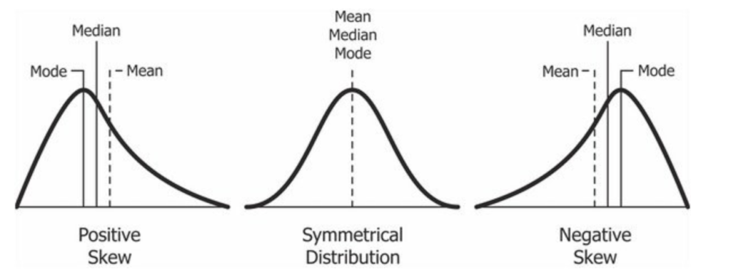
Note above that the relative position of the mean, median, and mode can be indicative of skew. Please also note that these values will rarely be exactly equal “in the real world”, and thus you need to weigh differences against the entire dataset when assessing skew. There is a lot of nuance like this in statistics; it is not always an “exact” science, but sometimes involves judgment calls and assessments based on what you observe in the data.
Using the starbucks dataset, we can look at some of these descriptive statistics to understand what is going on.
4.4.1 Notation
We use Greek lettering for populations and Roman lettering for samples. For example:
\(\sigma\) is a population, but \(s\) is a sample (both these variables refer to standard deviation).
\(\mu\) is a population, but \(\bar{x}\) is a sample (both of these variables refer to the mean).
4.4.2 Mean
The mean is the “average” value within a set of data, specifically, the sum of all values divided by the length of those values: \(\frac{\sum_{i=1}^nx}{n}\).
Click to see how to calculate Mean
head(starbucks)# A tibble: 6 × 2
Hour Frap_Num
<chr> <dbl>
1 0600-0659 2
2 0700-0759 3
3 0800-0859 2
4 0900-0959 4
5 1000-1059 8
6 1100-1159 7Here, we are specifically interested in the number of frappuccinos.
# get vector of frappuccino number
fraps <- starbucks$Frap_Num

# get mean of vector
mean(fraps)
[1] 6.222222Note that the above should be rounded to a whole number, since we were given the data in whole numbers!
mean(fraps) |>
  round(0)
[1] 6# OR
round(mean(fraps),0)[1] 6We already covered calculating the average manually in our previous tutorial, but we can do that here as well:
# sum values
# divide by n, length of vector
# round to 0 places
round(sum(fraps)/length(fraps),0)
[1] 6
4.4.3 Range
The range is the difference between the largest and smallest units in a dataset. I.e., it is the maximum value in a dataset minus the smallest value in a dataset.
Click to see how to calculate Range
We can use the commands min and max to calculate this.
max(fraps) - min(fraps)[1] 13The range of our dataset is 13.
NOTE that the R function range will not return the statistic of range, it will only return the maximum and minimum values from the dataset. This is not the correct answer when asked for the range for any homework or test questions.
range(fraps)[1] 2 15
4.4.4 Median
The median is also known as the 50th percentile, and is the midpoint of the data when ordered from least to greatest. If there are an even number of data points, then it is the average point between the two center points. For odd data, this is the \(\frac{n+1}{2}\)th observation. For even data, since we need to take an average, this is the \(\frac{\frac{n}{2}+(\frac{n}{2}+1)}{2}\).
Click to see how to calculate the Median
R has a default method for calculating median - median.
4.4.4.1 Odd number of values
# use default
median(fraps)
[1] 4Now, to calculate by hand:
length(fraps)[1] 9We have an odd length.
# order gets the order
order(fraps)
[1] 1 3 7 2 4 6 5 9 8# [] tells R which elements to put where
frap_order <- fraps[order(fraps)]
frap_order[1] 2 2 2 3 4 7 8 13 15# always use parentheses
# make sure the math maths right!
(length(frap_order)+1)/2[1] 5Which is the fifth element in the vector?
frap_order[5][1] 44.4.4.2 Even number of values
Given that we are trying to find the “middle” number, this is more complicated when using a vector that has an even number of values. Let’s calculate this by hand:
# remove first element
even_fraps <- fraps[-1]

even_fraps_order <- even_fraps[order(even_fraps)]

even_fraps_order
[1] 2 2 3 4 7 8 13 15median(even_fraps)[1] 5.5Now, by hand: \(\frac{\frac{n}{2}+(\frac{n}{2}+1)}{2}\).
n <- length(even_fraps_order)

# get n/2 position from vector
m1 <- even_fraps_order[n/2]
# get n/2+1 position
m2 <- even_fraps_order[(n/2)+1]

# add these values, divide by two for "midpoint"
med <- (m1+m2)/2

med
[1] 5.5As we can see, these values are equal!
4.4.5 Other quartiles and quantiles
We also use the 25th percentile (25%, 0.25) and the 75th percentile (75%, 0.75) to understand data distributions. These are calculated similar to the above, but the bottom quartile is only \(\frac{1}{4}\) of the way between values and the 75th quartile is \(\frac{3}{4}\) of the way between values. We can use the R function quantile to calculate these. Before implementing, please read this whole section - R has nine different methods for calculating the quantiles!
Click to see how to find Quartiles and Quantiles
R has a default function for finding quantiles which is called quantile.
quantile(frap_order) 0% 25% 50% 75% 100%
2 2 4 8 15 We can specify a quantile as well:
quantile(frap_order, 0.75)75%
8 We can also calculate these metrics by hand. Let’s do it for the even dataset, since this is more difficult.
quantile(even_fraps_order) 0% 25% 50% 75% 100%
2.00 2.75 5.50 9.25 15.00 Note that the 25th and 75th percentiles are also between two different values. These can be calculated as a quarter and three-quarters of the way between their respective values.
# 75th percentile

n <- length(even_fraps_order)

# get position
p <- 0.75*(n+1)

# get lower value
# round down
m1 <- even_fraps_order[trunc(p)]

# get upper value
# round up
m2 <- even_fraps_order[ceiling(p)]

# position between
# fractional portion of rank
frac <- p-trunc(p)

# calculate the offset from lowest value
val <- (m2 - m1)*frac

# get value
m1 + val
[1] 11.75Wait… why does our value differ?
R, by default, calculates quantiles using what is called Type 7, in which the quantiles are calculated by \(p_k = \frac{k-1}{n-1}\), where \(n\) is the length of the vector and \(k\) refers to the quantile being used. However, in our class and in many situations, we use Type 6 interpretation of \(p_k = \frac{k}{n + 1}\). Let’s try using Type 6:
quantile(even_fraps_order, type = 6) 0% 25% 50% 75% 100%
2.00 2.25 5.50 11.75 15.00 Now we have the same answer as we calculated by hand!
This is a classic example of how things in R (and in statistics in general!) can depend on interpretation and are not always “hard and fast” rules.
In this class, we will be using Type 6 interpretation for the quantiles - you will have to specify this in the quantile function EVERY TIME! If you do not specify Type 6, you will get the questions incorrect and you will get answers that do not agree with the book, with Excel, or what you calculate by hand.
4.4.6 Mode
The mode is the value which occurs most frequently within a dataset.
Click to see manual method
There is no default code to find the mode in R. We can do this by hand, by counting the number of occurrences of each value as shown below.
This method is based on the custom function for mode outlined by Statology.
# unique counts
u <- unique(fraps)
u
[1] 2 3 4 8 7 15 13# which elements match
match(fraps,u)[1] 1 2 1 3 4 5 1 6 7# count them
tab <- match(fraps,u) |>
tabulate()
tab[1] 3 1 1 1 1 1 1Get the highest value.
u[tab == max(tab)][1] 2Notice this uses ==. This is a logical argument that means “is equal to” or “is the same as”. For example:
2 == 2[1] TRUEThese values are the same, so TRUE is returned.
2 == 3[1] FALSEThese values are unequal, so FALSE is returned. R will read TRUE as 1 and FALSE as ZERO, such that:
sum(2 == 2)[1] 1and
sum(2 == 3)[1] 0This allows you to find how many arguments match your condition quickly, and even allows you to subset based on these indices as well. Keep in mind you can use greater than <, less than >, greater than or equal to <=, less than or equal to >=, is equal to ==, and is not equal to != to identify numerical relationships. Other logical arguments include:
&: both conditions must beTRUEto match (e.g.,c(10,20) & c(20,10)). Try the following as well:fraps < 10 & fraps > 3.&&: and, but works with single elements and allows for better parsing. Often used withif. E.g.,fraps < 10 && fraps > 3. This will not work on our multi-elementfrapvector.|: or, saying at least one condition must be true. Try:fraps > 10 | fraps < 3.||: or, but for a single element, like&&above.!: not, so “not equal to” would be!=.
However, the library UNKstats has many missing basic statistical functions, including find_mode(). Use this method in your code to reduce clutter and make the code run faster.
find_mode(fraps)[1] "Mode: 2"
[1] "Mode count: 3"The output of this function is two lines. The first line returns the value(s) for the mode, while the second line tells us the frequency with which this value occurs.
4.4.7 Variance
When we are dealing with datasets, the variance is a measure of the total spread of the data. The variance is calculated using the following:
\[\sigma^2=\frac{\sum (x_i-\bar{x})^2}{n-1}\]
Essentially, this means that for every value of \(x\), we are finding the difference between that value and the mean and squaring it, summing all of these squared differences, and dividing them by the number of samples in the dataset minus one.
Click to see how to calculate Variance
R has a built in function for variance - var.
var(frap_order) |>
  round(2)
[1] 24.44Click to see how to calculate Variance by hand
Let’s calculate the frap dataset variance by hand.
frap_order[1] 2 2 2 3 4 7 8 13 15Now to find the differences.
diffs <- frap_order - mean(frap_order)

diffs
[1] -4.2222222 -4.2222222 -4.2222222 -3.2222222 -2.2222222 0.7777778 1.7777778
[8] 6.7777778 8.7777778Note that R is calculating the same thing for the entire vector! Since these are differences from the mean, they should sum to zero.
sum(diffs)[1] 3.552714e-15This is not quite zero due to rounding error, but is essentially zero as it is 0.0000000000000036.
# square differences
diffs_sq <- diffs^2

diffs_sq
[1] 17.8271605 17.8271605 17.8271605 10.3827160 4.9382716 0.6049383 3.1604938
[8] 45.9382716 77.0493827Now we have the squared differences. We need to sum these and divide by \(n-1\).
n <- length(frap_order)

var_frap <- sum(diffs_sq)/(n-1)

var_frap
[1] 24.44444Let’s check this against the built-in variance function in R.
var(frap_order)[1] 24.44444They are identical! We can check this using a logical argument.
var_frap == var(frap_order)[1] TRUESeeing as this is TRUE, we calculated it correctly.
4.4.8 Standard deviation
The standard deviation (\(\sigma\)) is the square root of the variance, and is used to help describe the spread of datasets.
Click to see how to calculate standard deviation
sqrt(var_frap)[1] 4.944132There is also the built in sd function in R:
sd(frap_order)[1] 4.944132We can test the manual method against the built in sd function in R:
sqrt(var_frap) == sd(frap_order)[1] TRUEAs you can see, we calculated this correctly!
4.4.9 Standard error
The standard error is used to help understand the spread of data and to help estimate the accuracy of our measurements for things like the mean. The standard error is calculated thusly:
\[ SE = \frac{\sigma}{\sqrt{n}} \]
Click to see how to calculate standard error
There is not a built in function for standard error in R, but we can use UNKstats.
se(frap_order)[1] 1.648044Remember, the standard error is used to help reflect our confidence in a specific measurement (e.g., how certain we are of the mean, and what values we believe the mean falls between). We want our estimates to be as precise as possible with as little uncertainty as possible. Given this, does having more samples make our estimates more or less confident? Mathematically, what happens as our sample size increases?
4.4.10 Coefficient of variation
The coefficient of variation, another measure of data spread and location, is calculated by the following:
\[ CV = \frac{\sigma}{\mu}*100 \]
If we were to calculate this by hand, it would be done with this function:
val <- sigma/mu*100We can also use the function in UNKstats.
cv(frap_order) |>
  round(2)
[1] 79.46#Remember that we will need to round values.
4.4.11 Outliers
Click to see manual method
Outliers are any values that are outside of the 1.5 times the interquartile range. We can calculate this for our example dataset as follows:
lowquant <- quantile(frap_order,0.25,type = 6) |> as.numeric()

hiquant <- quantile(frap_order,0.75,type = 6) |> as.numeric()

iqr <- hiquant - lowquant
Click to see IQR method
We can also calculate the interquartile range using IQR. Remember, you must use type = 6!
iqr <- IQR(frap_order, type = 6)Now, to calculate the “whiskers”.
lowbound <- lowquant - (1.5*iqr)
hibound <- hiquant + (1.5*iqr)

# low outliers?
# select elements that match
# identify using logical "which"
frap_order[which(frap_order < lowbound)]numeric(0)# high outliers?
# select elements that match
# identify using logical "which"
frap_order[which(frap_order > hibound)]numeric(0)We have no outliers for this particular dataset.
Click to see DescTools method
This can also be done with DescTools.
# don't forget to install, if needed!
library(DescTools)

Outlier(frap_order)numeric(0)Again, there are no outliers as this code is effectively the same. If there are, it will return all outliers, but not indicate if they are high or low. This can be solved by comparing the returned outlier to the mean. If it is above the mean, it is a high outlier, and vice versa.
4.5 Homework: Descriptive Statistics
Now that we’ve covered these basic statistics, it’s your turn!
4.5.1 Homework instructions
Please create an RMarkdown document that will render as an .html file. You will submit this file to show your coding and your work. Please refer to the Introduction to R for refreshers on how to create an .html document in RMarkdown.
Please show all of your work for full credit.
4.5.2 Data for homework problems
For each question, calculate the mean, median, range, interquartile range, variance, standard deviation, coefficient of variation, standard error, and whether there are any “outliers”.
Please also write your own short response to the Synthesis question posed, which will involve thinking about the data and metrics you just analyzed.
4.5.2.1 1: UNK Nebraskans
Ever year, the university keeps track of where students are from. The following are data on the umber of students admitted to UNK from the state of Nebraska:
# create dataset in R
nebraskans <- c(5056,5061,5276,5244,5209,
                5262,5466,5606,5508,5540,5614)

years <- 2023:2013

nebraskans_years <- cbind(years,nebraskans) |>
  as.data.frame()

nebraskans_years
years nebraskans
1 2023 5056
2 2022 5061
3 2021 5276
4 2020 5244
5 2019 5209
6 2018 5262
7 2017 5466
8 2016 5606
9 2015 5508
10 2014 5540
11 2013 5614Using these data, please calculate the mean, median, range, interquartile range, variance, standard deviation, coefficient of variation, standard error, and whether there are any “outliers” for the number of UNK students from Nebraska.
In order to do this, we will need to first select the column that denotes the number of Nebraskans from the dataset. Remember, we need to save this as an object in R to do the analyses. Here is a demonstration of getting the column to look at the mean, so that you can repeat this for the other questions. This relies heavily on the use of $, used to get the data from a specific column.
# $ method
nebraskans <- nebraskans_years$nebraskans

nebraskans
[1] 5056 5061 5276 5244 5209 5262 5466 5606 5508 5540 5614Now we can get the mean of this vector.
mean(nebraskans) |>
  round(0) # don't forget to round!
[1] 5349Now, calculate the following for nebraskans:
mean -
mean()25th and 50th percentiles -
quantile()median -
median()range -
max()-min()interquartile range -
IQR()variance -
var()standard deviation -
sd()coefficient of variation -
cv()function defined abovestandard error -
sd()whether there are any “outliers” -
Outliers()
Synthesis question: Do you think that there are any really anomalous years? Do you feel data are similar between years? Note we are not looking at trends through time but whether any years are outliers.
4.5.2.2 2: Piracy in the Gulf of Guinea
The following is a dataset looking at oceanic conditions and other variables associated with pirate attacks within the region between 2010 and 2021 (Moura et al. 2023). Using these data, please calculate the mean, median, range, interquartile range, variance, standard deviation, coefficient of variation, standard error, and whether there are any “outliers” for distance from shore for each pirate attack (column Distance_from_Coast).
pirates <- read_csv("https://figshare.com/ndownloader/files/42314604")New names:
Rows: 595 Columns: 40
── Column specification
──────────────────────────────────────────────────────── Delimiter: "," chr
(18): Period, Season, African_Season, Coastal_State, Coastal_Zone, Navi... dbl
(20): ...1, Unnamed: 0, Year, Month, Lat_D, Lon_D, Distance_from_Coast,... dttm
(2): Date_Time, Date
ℹ Use `spec()` to retrieve the full column specification for this data. ℹ
Specify the column types or set `show_col_types = FALSE` to quiet this message.
• `` -> `...1`Now, calculate the following for Distance_from_Coast:
mean
median
25th and 75th percentiles
range
interquartile range
variance
standard deviation
coefficient of variation
standard error
whether there are any “outliers”
Synthesis question: Do you notice any patterns in distance from shore? What may be responsible for these patterns? Hint: Think about what piracy entails and also what other columns are available as other variables in the above dataset.
4.5.2.3 3: Patient ages at presentation
The following is a dataset on skin sores in different communities in Australia and Oceania, specifically looking at the amount of time that passes between skin infections (Lydeamore et al. 2020a). This file includes multiple different datasets, and focuses on data from children in the first five years of their life, on household visits, and on data collected during targeted studies (Lydeamore et al. 2020b).
ages <- read_csv("https://doi.org/10.1371/journal.pcbi.1007838.s006")Rows: 17150 Columns: 2
── Column specification ────────────────────────────────────────────────────────
Delimiter: ","
chr (1): dataset
dbl (1): time_difference
ℹ Use `spec()` to retrieve the full column specification for this data.
ℹ Specify the column types or set `show_col_types = FALSE` to quiet this message.Let’s see what this file is like real fast. We can use the command dim to see the rows and columns.
dim(ages)[1] 17150 2As you can see, this file has only two columns but 17,150 rows! For the column time_difference, please calculate the mean, median, range, interquartile range, variance, standard deviation, coefficient of variation, standard error, and whether there are any “outliers”.
Calculate the following for the time_difference:
mean
median
25th and 75th percentiles
range
interquartile range
variance
standard deviation
coefficient of variation
standard error
whether there are any “outliers”
Synthesis question: Folks will often think about probabilities of events being “low but never zero”. What does that mean in the context of secondary infection? What about these data make you think that a secondary infection is always possible?