remotes::install_github("CalebRother/UNKstats")18 Functions & Glossary
18.1 Installing UNKstats
18.2 Rounding & Formatting
As a reminder, we are following the rounding rules of the Auk and Condor (now Ornithology and Ornithological Applications).
Specifically, these rules are as follows:
No naked decimals (except for caliber):
Preface all decimals with a leading zero; \(0.002\) is correct, \(.002\) is incorrect.
For caliber, such as with weapons, never have a leading zero; ex., .45 bullet.
Use the same number of decimals as the original data or the precision of the instrument:
- Ex., if precision is \(0.01\), then all values should be rounded to hundredths.
Use the same number of decimals for values and uncertainties:
- Ex., \(45 \pm 4\), \(45.2 \pm 3.8\).
Round percentages to whole numbers* (or to one decimal):
- For this class, can round to one decimal, but in the referenced publications always round to whole number. You will never miss points for rounding percentage to a whole number.
All test statistics should be rounded to two (2) decimal places:
- \(F\), \(t\), \(p\), \(\tau\), \(\chi^2\), etc. should all be rounded to two decimal places.
All test statistics should show degrees of freedom:
For values with one degree of freedom, list like \(t_{(9)}=1.56\).
For values with multiple, list them; for ANOVA, put the degrees of freedom for Sum of Squares Between before degrees of freedom for Degrees of Error Within, like \(F_{(5,43)}=5.23\).
Round P-values as follows:
\(P \ge 0.01\): round to two decimal places like \(P = 0.24\).
\(0.01 > P \ge 0.001\): round to three decimal places like \(P = 0.005\).
\(0.001 > P \ge 0.0001\): round to four decimal places like \(P = 0.0007\).
\(P < 0.0001\): list exactly as \(P < 0.0001\).
- DO NOT list without spaces, or as \(P<.0001\)
18.3 Plaintext formatting
18.3.1 Equations
For equations, put $ on either side of the equation being typed. For example:
$4$ becomes \(4\) and $pi$ becomes \(\pi\).
Subscripts:
$Z_{34}$becomes \(Z_{34}\)Superscripts:
$Z^2$becomes \(Z^2\)Fractions:
$\frac{1}{2}$becomes \(\frac{1}{2}\)Common letters and commands:
\(\alpha\):
\alpha\(\beta\):
\beta\(\sigma\):
\sigma
18.3.2 In-line code
You can also put code within your plain text. For example, consider the following entered code text and the following output:
Here is an example of in line code: 3.5.Here is an example of in line code: 3.5.
18.4 Common Commands
The following are common useful commands used in R, with examples of their use.
Commands are given as Windows & Linux / Mac.
18.4.1 The basics
Save your file with
CTRL+S/ ⌘ +SUndo your last action with
CTRL+Z/ ⌘ +ZCut text with
CTRL+X/ ⌘ +XCopy text with
CTRL+C/ ⌘ +CPaste text with
CTRL+V/ ⌘ +VSelect all text in a document with
CTRL+A/ ⌘ +A
18.4.2 Code basics
A code chunk can be inserted using
CTRL+SHIFT+I/ ⌘ +shift+IRun a line of code with
CTRL+ENTER/ ⌘ +returnRun a code chunk with
CTRL+SHIFT+ENTER/ ⌘ +shift+returnRun all code in the document above where you were
CTRL+SHIFT+ALT+P/ ⌘ +shift+ ⌥ +PRun all code with
CTRL+ALT+R/ ⌘ + ⌥ +R
18.4.3 Code formatting
<-- save a value as an object. On Mac, the keyboard shortcut is ⌥ +-. Windows can be formatted so that the shortcut isALT+-.
x <- 10
x
[1] 10|>- “pipe” a command or output into another command. You can use the shortcutCTRL+SHIFT+M/ ^ +SHIFT+M.
# make repeatable
set.seed(930)

# random string
x <- rnorm(20)

x |>
  # pass to summary
  summary() |>
  # pass summary through round
  round(2)
Min. 1st Qu. Median Mean 3rd Qu. Max.
-1.94 -0.48 -0.06 -0.05 0.36 1.80 ->- save a value as an object at the end of a pipeline
# same pipeline as previous, but more sequential

# get random values
rnorm(20) |>
  # pass to summary
  summary() |>
  # pass summary through round
  round(2) ->
  # save as x
  x

x
Min. 1st Qu. Median Mean 3rd Qu. Max.
-2.60 -0.77 -0.24 -0.18 0.57 1.73 c- concatenate, place two values together
x <- c(10,11)
x
[1] 10 1118.4.4 Boolean logic
In order to create arguments in R, such as commands like which, we need to use Boolean logic commands.
For this example, I will create a string from 1 to 10 to perform the commands on. Note that I am using brackets [ ] to call out an index within the object using these commands.
These are as follows:
# example string
x <- 1:10>: greater than
x[x > 5][1] 6 7 8 9 10<: less that
x[x < 5][1] 1 2 3 4>=: greater than or equal to
x[x >= 5][1] 5 6 7 8 9 10<=: less than or equal to
x[x <= 5][1] 1 2 3 4 5==: is equal to
x[x == 5][1] 5|: or
x[x < 3 | x > 7][1] 1 2 8 9 10&: and
x[x > 3 & x < 7][1] 4 5 618.5 Basic statistics
Click here for basic statistics
For these examples, we will create a random vector of number to demonstrate how they work.
# make repeatable
set.seed(8675309)
# get random normal values
x <- rnorm(1000)mean- get the mean / average of a set of data
mean(x)[1] -0.02659863median(x)[1] -0.0006443188IQR(x)[1] 1.378508range(x)[1] -3.449557 3.412794# calculate range
abs(range(x)[1] - range(x)[2])[1] 6.862351# calculate range
max(x) - min(x)[1] 6.862351hist(x)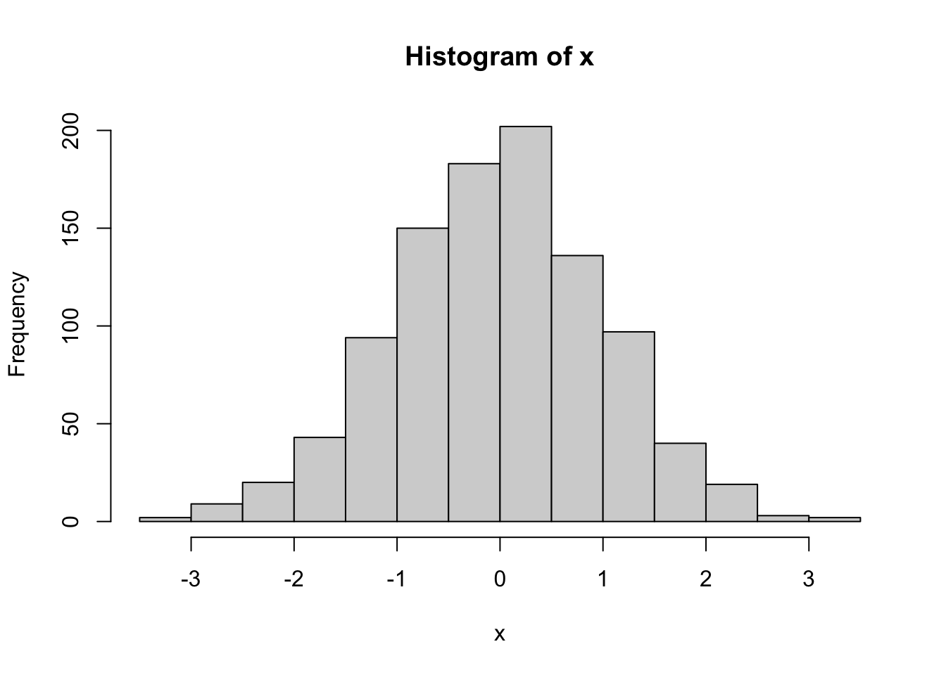
18.6 Null hypotheses
Click here for null hypotheses
18.6.1 \(\chi^2\) tests
18.6.1.1 \(\chi^2\) goodness-of-fit
\(H_0\): The frequency of observations fits the expected observation frequencies.
18.6.1.2 \(\chi^2\) test of independence (i.e., association)
\(H_0\): Variable X and Variable Y are not related.
18.6.2 One-sample tests
18.6.2.1 One-sample \(t\)-test
\(H_0\): \(\mu=X\)
18.6.2.2 Paired \(t\)-test
\(H_0\): \(\mu_1-\mu_2=0\) or \(\mu_d=0\)
18.6.2.3 Two-sample \(t\)-test
\(H_0\): \(\mu_1=\mu_2\)
18.6.3 Multi-sample tests
All ANOVA tests have essentially the same null hypotheses, with the primary null hypothesis being that all means are the same. Secondary hypotheses may exist about which means are different; we have to do a post-hoc test to determine which means are different.
\(H_0\): \(\mu_1=\mu_2=\mu_3=...=\mu_n\)
18.6.4 Correlation
For all correlation tests, the null is that the correlation is 0 (i.e., not correlated positively or negatively). You can get the \(p\) value for a test from a \(t\) distribution.
As an example, Pearson’s correlation:
\(H_0\): \(\rho = 0\)
18.6.5 Regression
\(H_0\): \(\beta = 0\)
where \(\beta\) is the slope.
18.7 Reshaping data
Consider the default iris dataset in R.
head(iris) Sepal.Length Sepal.Width Petal.Length Petal.Width Species
1 5.1 3.5 1.4 0.2 setosa
2 4.9 3.0 1.4 0.2 setosa
3 4.7 3.2 1.3 0.2 setosa
4 4.6 3.1 1.5 0.2 setosa
5 5.0 3.6 1.4 0.2 setosa
6 5.4 3.9 1.7 0.4 setosaThis data frame is in “long format”, where the grouping variables are all in a single column. This is the format R prefers, but it is harder for humans to do statistics on it. Humans prefer “wide” data for a single variable. Let’s consider a subset of the dataframe for only Sepal.Length.
iris_sepal_length <- iris |>
  select(Species, Sepal.Length)

head(iris_sepal_length)
Species Sepal.Length
1 setosa 5.1
2 setosa 4.9
3 setosa 4.7
4 setosa 4.6
5 setosa 5.0
6 setosa 5.4The above is in “long format”. We can now transition to “wide format” using pivot_wider.
iris_wide <- iris_sepal_length |>
  # add ID column if needed
  # add ID number by explanatory variable
  # here, that is "Species"
  mutate(id = row_number(), .by = Species) |>
  pivot_wider(names_from = Species,
              values_from = Sepal.Length,
              id_cols = id)

head(iris_wide)
# A tibble: 6 × 4
id setosa versicolor virginica
<int> <dbl> <dbl> <dbl>
1 1 5.1 7 6.3
2 2 4.9 6.4 5.8
3 3 4.7 6.9 7.1
4 4 4.6 5.5 6.3
5 5 5 6.5 6.5
6 6 5.4 5.7 7.6We can also convert back to “long format” for ease with R.
iris_long <- iris_wide |>
  pivot_longer(!id, names_to = "Species", values_to = "Sepal.Length")

head(iris_long)
# A tibble: 6 × 3
id Species Sepal.Length
<int> <chr> <dbl>
1 1 setosa 5.1
2 1 versicolor 7
3 1 virginica 6.3
4 2 setosa 4.9
5 2 versicolor 6.4
6 2 virginica 5.818.8 Custom functions from class and elsewhere
18.8.1 Normal distributions
18.8.2 ANOVA
Click here for ANOVA functions
The following example data are going to be used to illustrate these functions.
#### EXAMPLE DATA ####
set.seed(8675309)

for(i in 1:4){
  x <- rnorm(10)
  if(i == 1){
    x <- rnorm(10, mean = 2)
    data <- x |> as.data.frame()
    colnames(data) <- "Response"
    data$Explanatory <- paste0("x",i)
  }else{
    newdat <- x |> as.data.frame()
    colnames(newdat) <- "Response"
    newdat$Explanatory <- paste0("x",i)
    data <- rbind(data,newdat)
  }
}

# split into "typical" table
expanded_data <- NULL
expanded_data$x1 <- data$Response[which(data$Explanatory=="x1")]
expanded_data$x2 <- data$Response[which(data$Explanatory=="x2")]
expanded_data$x3 <- data$Response[which(data$Explanatory=="x3")]
expanded_data$x4 <- data$Response[which(data$Explanatory=="x4")]

expanded_data <- expanded_data |>
  as.data.frame()
The above is a one-way ANOVA. As a reminder, we would calculate the test as follows:
# pivot longer does not work for one-way ANOVA, requires blocking factor
# can rbind things with same colnames to make longer

example_aov <- aov(Response ~ Explanatory, data)

summary(example_aov)
Df Sum Sq Mean Sq F value Pr(>F)
Explanatory 3 23.40 7.801 11.54 1.89e-05 ***
Residuals 36 24.33 0.676
---
Signif. codes: 0 '***' 0.001 '**' 0.01 '*' 0.05 '.' 0.1 ' ' 1Above, we can see a significant result of the ANOVA. We can follow this up with a Tukey test. This requires the package agricolae! Check the ANOVA pages, however, as not all ANOVA can use this agricolae shortcut method.
example_tukey <- HSD.test(example_aov,
                          # what to group by?
                          "Explanatory",
                          # significance level?
                          alpha = 0.05,
                          # are data unbalanced
                          unbalanced = FALSE,
                          # show answer?
                          console = TRUE)
Study: example_aov ~ "Explanatory"

HSD Test for Response

Mean Square Error:  0.6758192

Explanatory,  means

     Response       std  r        se        Min      Max        Q25         Q50
x1  1.7620153 1.0505466 10 0.2599652  0.4504476 3.972459  1.1175485  1.44911720
x2  0.2841495 0.7532422 10 0.2599652 -0.4729986 1.985826 -0.3497379  0.21347543
x3  0.2197337 0.7019368 10 0.2599652 -0.6150452 1.574903 -0.2436023 -0.04493909
x4 -0.2890524 0.7345336 10 0.2599652 -1.9769014 0.684072 -0.5394534 -0.07741642
          Q75
x1 2.07491533
x2 0.64579865
x3 0.53544151
x4 0.04323417

Alpha: 0.05 ; DF Error: 36
Critical Value of Studentized Range: 3.808798

Minimun Significant Difference: 0.9901551

Treatments with the same letter are not significantly different.

     Response groups
x1  1.7620153      a
x2  0.2841495      b
x3  0.2197337      b
x4 -0.2890524      b
18.8.2.1 Summarize data (for plotting)
Remember - you need to change "Explanatory" to your explanatory variable (in quotes!) and you need to change Response to your response column (no quotes!). The following requires plyr to work, but the function itself should call up plyr if you do not yet have it loaded.
# summarize by group
summary_data <- function(data, explanatory){
  require(plyr)
  ddply(data, paste(explanatory), summarise,
                 N = length(Response),
                 mean = mean(Response),
                 sd = sd(Response),
                 se = sd / sqrt(N))
}

example_summary <- summary_data(data = data, explanatory = "Explanatory")
Loading required package: plyr------------------------------------------------------------------------------You have loaded plyr after dplyr - this is likely to cause problems.
If you need functions from both plyr and dplyr, please load plyr first, then dplyr:
library(plyr); library(dplyr)------------------------------------------------------------------------------
Attaching package: 'plyr'The following objects are masked from 'package:dplyr':
arrange, count, desc, failwith, id, mutate, rename, summarise,
summarizeThe following object is masked from 'package:purrr':
compactexample_summary Explanatory N mean sd se
1 x1 10 1.7620153 1.0505466 0.3322120
2 x2 10 0.2841495 0.7532422 0.2381961
3 x3 10 0.2197337 0.7019368 0.2219719
4 x4 10 -0.2890524 0.7345336 0.232279918.8.2.2 Significant label maker
This command requires a Tukey HSD object from agricolae. You can manually create a table like this for some other scenarios; see relevant pages for documentation.
# note first group must be EXACT MATCH to your summary_data object
# groups are saved in the Tukey object
# this is true for Tukey later as well

# the following is a function that will make the significant label table
sig.label.maker <- function(tukey_test, group_name){
  sig.labels <- tukey_test$groups |>
    # convert to a data.frame
    as.data.frame() |>
    # create a new column - place rownames into the column
    # converts to a format better for ggplot
    mutate(Explanatorys = rownames(tukey_test$groups)) |>
    # rename column to prevent confusion
    # specify dplyr; default function may be from plyr and not work
    dplyr::rename(Significance = groups)
  colnames(sig.labels)[which(colnames(sig.labels) == "Explanatorys")] <- group_name
  return(sig.labels)
}

# Function requires explanatory groups in quotes
sig_labels <- sig.label.maker(example_tukey, "Explanatory")

sig_labels
Response Significance Explanatory
x1 1.7620153 a x1
x2 0.2841495 b x2
x3 0.2197337 b x3
x4 -0.2890524 b x418.8.2.3 ANOVA plotter
The following function plots ANOVAS if you have a summary_data object and a sig_labels object, as shown above. This does not work on ANOVA with interactive components.
anova_plotter <- function(summary_data, explanatory,
                          response, sig_labels,
                          y_lim=NA, label_height=NA,
                          y_lab=NA, x_lab=NA){
  require(tidyverse)

  plot_data_1 <- summary_data[,c(explanatory, response, "se")]
  plot_data_2 <- sig_labels[,c(explanatory,"Significance")]

  colnames(plot_data_1) <- c("explanatory", "response", "se")
  colnames(plot_data_2) <- c("explanatory", "Significance")

  plot_data <- plot_data_1 |>
    full_join(plot_data_2, by = "explanatory")

  if(is.na(y_lim)){
    if(min(plot_data$response) < 0){
      y_lim <- c(min(plot_data$response) -
          4*max(plot_data$se),
        max(plot_data$response) +
          4*max(plot_data$se))
    }else{
      y_lim <- c(0,max(plot_data$response) +
                                4*max(plot_data$se))
    }
  }
  if(is.na(label_height)){label_height <- 0.25*max(y_lim)}
  if(is.na(y_lab)){y_lab <- "Response"}
  if(is.na(x_lab)){x_lab <- "Treatment"}

  plot_1 <- ggplot(plot_data,
         aes(x = explanatory, y = response)) +
    geom_point() +
    geom_errorbar(data = plot_data,
                  aes(ymin = response - 2*se,
                      ymax = response + 2*se,
                      width = 0.1)) +
    ylim(y_lim) +
    theme_classic() +
  theme(legend.position = "none",
        axis.text.x = element_text(angle = 90, vjust = 0.5, size = 5)) +
  geom_text(data = plot_data,
            # make bold
            fontface = "bold",
            # define where labels should go
            aes(x = explanatory,
                # define height of label
                y = label_height,
                # what are the labels?
                label = paste0(Significance))) +
  xlab(x_lab) +
  ylab(y_lab)

  print(plot_1)
}

anova_plotter(summary_data = example_summary,
              explanatory = "Explanatory",
              response = "mean", # from summary_data table! What is to be plotted
              sig_labels = sig_labels)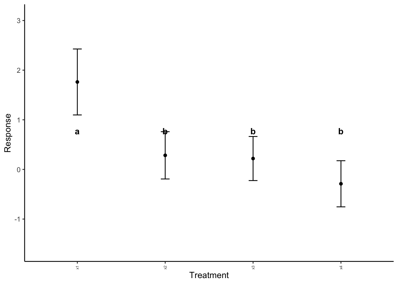
Note that in the above, the default label height is not working for us. We can adjust this with label_height.
anova_plotter(summary_data = example_summary,
              explanatory = "Explanatory",
              response = "mean", # from summary_data table! What is to be plotted
              sig_labels = sig_labels,
              label_height = -1)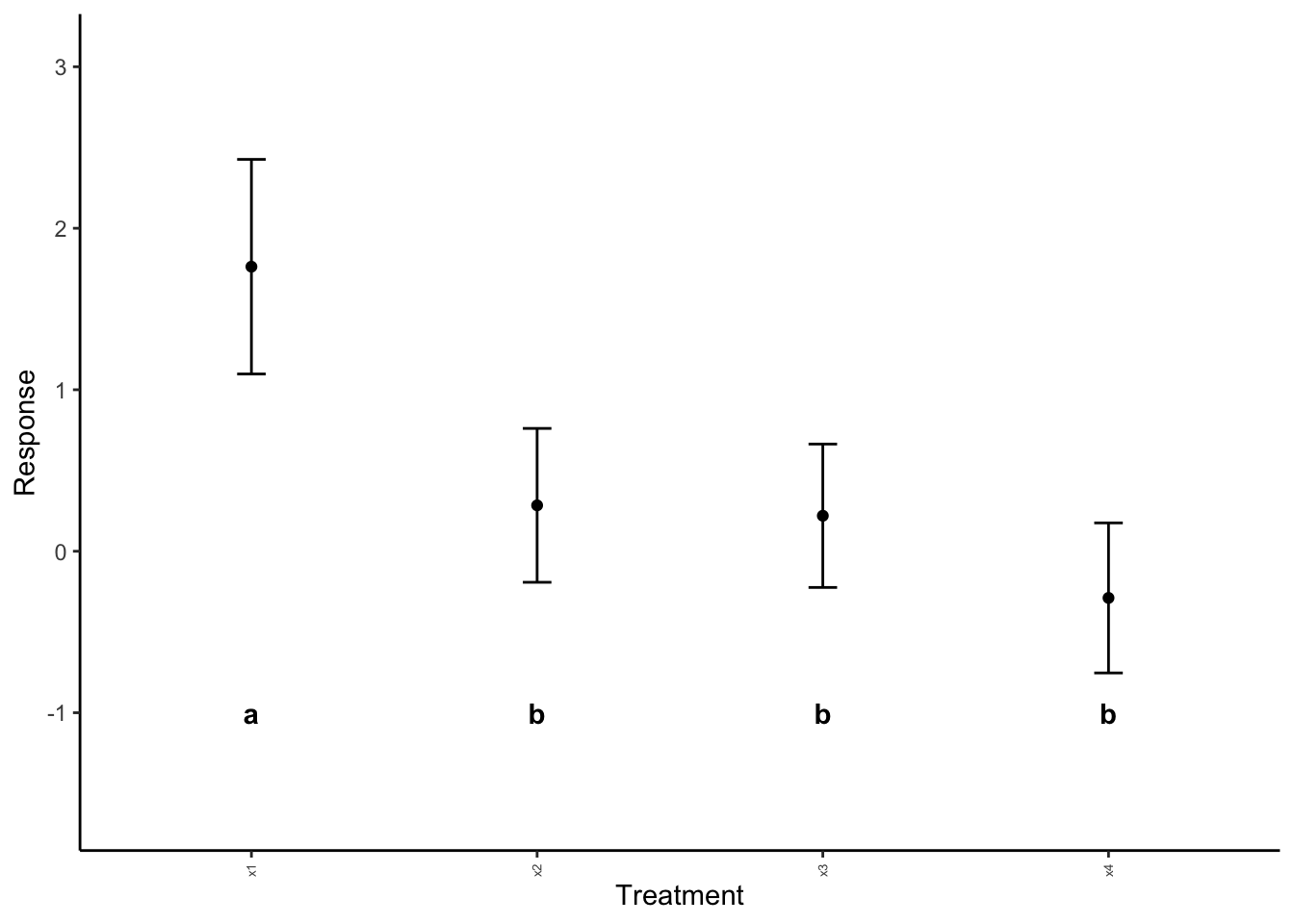
Much better!